Dog Breed Classifier
Image Classification using Transfer Learning
The code used for this project can be viewed as a jupyter notebook. A full project submission can be viewed here, or a more in-depth notebook detailing the model training process can be found here. If you would like access to the actual notebooks, they can be found in the project’s GitHub repository.
Project Overview
This project was part of Udacity’s Artificial Intelligence Nanodegree. The goal of the project was to create a pipeline that takes an image and detects whether a human or dog is present, predicting the breed for the dog or deciding what dog breed the human looks similar to. The figure below outlines this process.
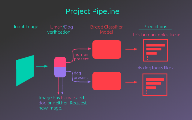
As shown above, there is an input image which goes through the human/dog verification process. This was broken up into two separate steps:
- Human Verification - To determine if a human is present in the image, a pre-trained haar cascade face detector from the OpenCV library was used.
- Dog Verification - For dog verification, a full pre-trained version of ResNet-50 was used. This model is available in Keras with weights pre-trained on the ImageNet dataset. The images in the ImageNet data set are divided into 1000 categories with several of these categories being dogs of different breeds. Making use of this, the model was used as a dog detector, by having the model predict the ImageNet class of the image. If the class falls into one of the dog breed categories, then a dog is present.
Once it has been confirmed that a human or a dog is present in the image, it is then passed to the breed classification model to determine what breed the human or dog most resembles. The predictions are printed out along with whether a human or dog was detected. If the image was found to contain both a human and a dog, or neither, a new image is requested. The breed classification model is most accurate when classifying on a single entity.
While the pre-trained ImageNet models do allow for some dog breed classification, these models are not specifically tuned to distinguish between the dog breeds. A better model can be made by training for this specific task.
The Breed Classification Model
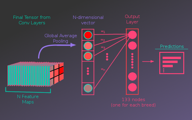
Building this dog breed classification model was the main focus of this project. Even through the pre-trained ImageNet models are not optimally tuned for this task, they will still be extremely useful in building the dog breed classifier. The models trained on ImageNet are very good at extracting features from images. Luckily, the images for this task are similar to the images of ImageNet. These models use convolutional neural networks to extract the image features and they can be used in this new model by transferring what the pre-trained models have already learned. The following figure shows a basic summary of the breed classification model.
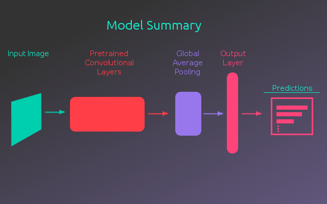
The basic idea for this model’s architecture is to use the convolutional layers from a pre-trained model to extract the features from the input image. These features are distilled down to a single vector using a Global Average Pooling layer. This vector is passed to a fully-connected output layer that calculates the probability for each dog breed.
The following figure illustrates what is happening in the convolutional layers. The model starts with an input image which is represented as a 3-D tensor (3 color channels x Width X Height). A convolutional layer convolves over the image tensor with N different kernels(a matrix of weights). These kernels look for various features in the image. Ultimately, this produces a new 3-D tensor (N feature channels x Output Width x Output Height). These layers are chained together with the output of one convolutional layer feed as input into the next convolutional layer. If you are not familiar with how the kernel calculation works, this blog post has a very good visual explanation of what is happening.
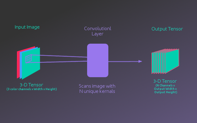
The convolutional layers of the models trained on ImageNet have learned useful weights for the kernels they use, allowing them to detect distinguishing features of real world objects. The first few convolutional layers are able to pick up on simple objects(textures, edges, shapes) at high resolution, and by chaining these layers together, later layers are able to detect higher level objects(eyes, noses, ears). However, this comes at the cost of spatial resolution. The effect after passing an image through the convolutional layers is that the 3-D tensor representing the image is transformed into a 3-D tensor that has a smaller width and height, but many high level feature maps that show what regions of the image have certain features.
For this model the pre-trained convolutional layers output a final tensor with N feature maps. If it is unclear what the feature maps actually represent, an example would be: if a given feature detector(kernel) is looking for eyes, it will output high values for regions of the image where eyes might be present and low values for regions where eyes are not likely. Now, the pre-trained models were not specifically told to have eye detectors, they learned what kind of detectors are useful through the training process. Anyway, these feature maps are passed through a Global Average Pooling layer, which averages the values of each feature map into a single value. This produces a vector, N-entries long, where each entry represents the average value of a feature map. Feature maps with higher values mean the image is more likely to have those features(only the model really knowing what those features are).
So, this vector of feature values is passed to a fully connected layer, where each node represents the probability that the image contains a certain dog breed. The way it calculates this is by taking a weighted sum of the values in the feature vector for each node and then these values are put through a softmax function constraining the sum of the nodes to equal 1. This converts the node values into a probability for each breed. The training process for the model is to tune the weights in the weighted sum, such that the model learns what features are important when distinguishing each breed.
This process is illustrated below:
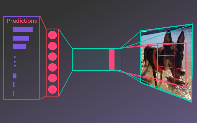
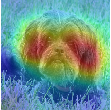
This model architecture has several nice effects. First, it is relatively simple so the model is less likely to over fit and takes up less memory. In contrast, a model might have several fully connected layers, between the convolutional features and the output layer. Secondly, because the output nodes associated with the breeds connect directly to the feature maps, we can visualize what the model is ‘seeing’. By plotting all the feature maps over the original image and weighting each map by the weights from the predicted breed, a saliency map can be produced. This shows what regions of the image contributed the most to the final prediction. Below we have the saliency map produced for the image of a Lhasa Apso dog, which the model mistakenly predicts as a Havenese(although Lhasa Apso was the 2nd highest prediction). The saliency map shows that the ears appear to strongly influence the models decision.
Evaluation and Performance
Using the model architecture described above, several different pre-trained convolutional layers were tested. Keras has several different models that can be loaded with pre-trained weights. The models tested include:
- VGG16
- VGG19
- ResNet50
- InceptionV3
- Xception
- Inception-ResNetV2
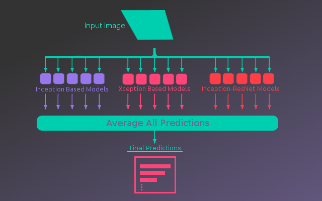
The Inception based models(InceptionV3, Xception, and Inception-ResNetV2) produced that best performance, achieving close to 90% accuracy on the test data. This was noticeably higher than the other models which were down around 80% accuracy. Using these models an ensemble was built. For each type of pretrained model, the convolutional layers were used to build 5 full models. The predictions from these 15 models were then averaged to give a final prediction. This improved the accuracy another 3-4%, up to 93.6% on the final test set. Below is an illustration of the ensemble architecture.
Summary and Further
The final model was able to produce 93.6% accuracy classifying on 133 breeds. In comparison to the state of the art, Kaggle had a similar competition, recently after this project was completed, where top teams were achieving 98% accuracy. However, this was on a different dataset, classifying over 120 breeds with access to larger amounts of data. Given access to more data, this model would most likely have improved. With the dataset used, the model only had ~70 images per breed to learn from.
If this project was extended there are several additional avenues for improved performance. Of the misclassified breeds, there were a large number where the predicted breed and the actual breed are extremely hard to distinguish, even by humans. It might be possible to build separate models that predict over a certain group of dogs. For example, one of the model’s mis-classifications was confusing a Cardigan Welsh Corgi with a Pembroke Welsh Corgi. There might be an improvement if a separate model to distinguish Corgi’s was trained and used in the case that a predicted breed fell into the corgi group. This however would add quite a lot of time and memory usage to the prediction pipeline.
Another possible avenue would be to use an R-CNN(Region Convolutional Neural Network). With a region based network, the model predicts what parts of the image it should look at. This would allow the model to focus in specifically on the dog, removing any ‘noise’ information from the background of the image. This would also have an added bonus that it could be used as the human/dog verification step. Overall, the model performance is quite impressive and adequate, as is, for the given task. If you are interested in seeing the model’s training process and code, please check out the notebooks linked at the beginning of the article.