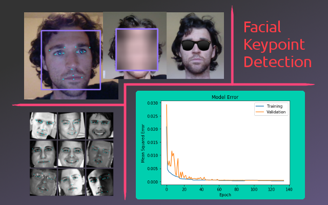
Facial Key Point Detection
Capstone Project of Udacity's Artificial Intelligence Nanodegree
The code used for this project can be viewed as a Jupyter notebook. The full project submission can be viewed here. If you would like access to the actual notebook, they can be found in the project’s GitHub repository.
Overview
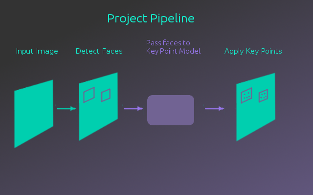
In this final project for Udacity’s AIND, the goal was to create a facial key point detection model. This model was then integrated into a full pipeline that takes an image, identifies any faces in the image, then detects the key points of those faces.
Preprocessing with OpenCV
Part of this project was to become familiar with the OpenCV library. Specifically, to use it in preprocessing the input images. In the case of this project, it was used to convert the image to gray scale and detect faces in the image. Another useful feature of OpenCV is Gaussian blurring, which can be used to conceal the identity of a detected face.
The following figure shows the result of applying face detection and Gaussian blurring to an image.
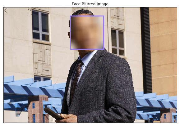
Using the face detector from the OpenCV library, faces in an image can then be cropped to be fed into the key point detection model.
Dataset
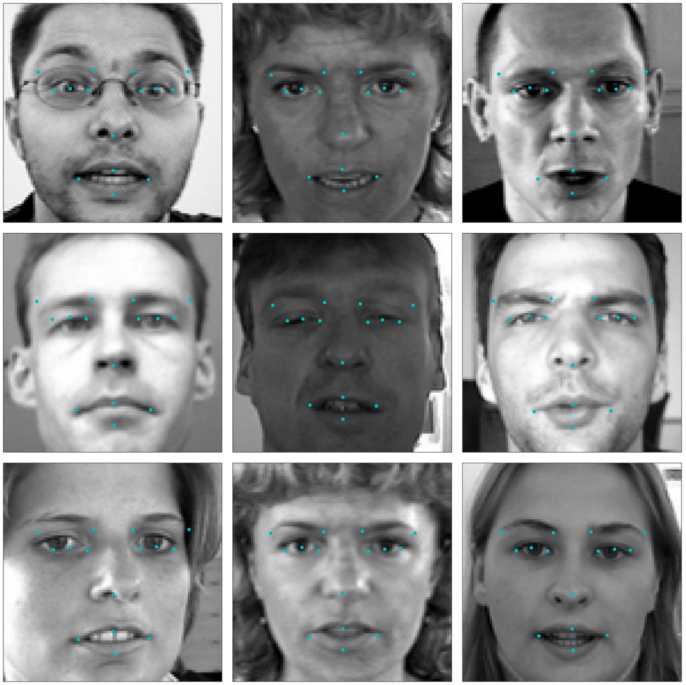
To train the key point detection model, a dataset of faces with corresponding key point labels was used. This dataset comes from Kaggle, consisting of 96x96 gray scale images of faces with 15 (x,y) coordinates labeling the facial key points. The original dataset contained 7049 images, however not all the images had the full 15 key point labels. To deal with this, only the images with the full 15 key points were used. This left 2140 images, 500 of which were split into a test set. The following figure shows a sample of the dataset.
Augmentation
With a relatively small training set of 1640 images, the data was augmented in several ways to increase the number of example images the model could learn from. This was made slightly more challenging by the fact that not only did the input images need to be augmented, but the key point labels also had to be augmented so they matched the same point on the newly augmented image. Two types of augmentation were applied, the code outlining this process can be found in the projects Jupyter notebook.
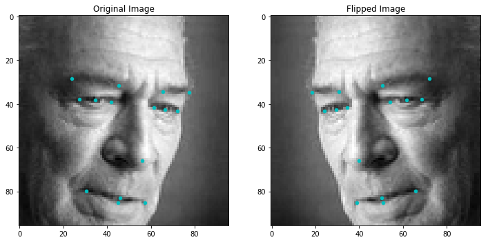
Horizontal Flipping - This was relatively straight forward. The x values of the images and the key points were reflected over the center of the image. Key points corresponding to the left side of the face were swapped with the corresponding right key point. This doubled the training data. Below is an example of the horizontal flipping.
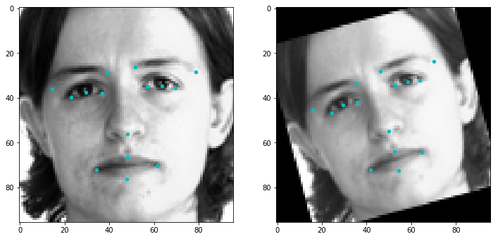
Rotation and Scaling - Rotation and scaling was a bit more challenging, but thanks to OpenCV it was easy to construct a rotation/scaling matrix which was applied to both the image and its key points. Adding a rotated/scaled version of the dataset onto the normal dataset doubled the training examples again. Below is an example of this augmentation.
After augmenting the original dataset, the model now had 6560 examples to train on.
Building the Model
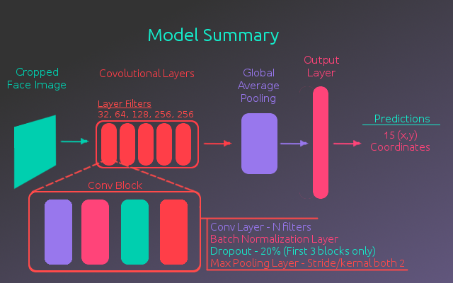
The architecture used for this model was loosely based on the VGG16 model, a convolutional neural network built for classifying on ImageNet. The VGG16 model uses 5 convolutional blocks to extract features from an image. These blocks consist of several convolutional layers followed by a max pooling layer, where the image dimensions are reduced in half. In the model used for this project each convolutional block only has one convolutional layer. The reasoning for this is that with the limited amount of data, a simpler model was less likely to over fit.
In addition to using fewer convolutional layers, dropout layers were added to the first 3 convolutional blocks with a dropout rate of 20% and batch normalization layers were added after each convolutional layer. Both of these newer techniques were absent from the original VGG16 network and help prevent over fitting.
Using this architecture to extract the image features, the output of the convolutional layers was fed to a Global Average Pooling layer and then to a fully connected output layer of 30 nodes(x,y values for each of 15 key points). The following figure illustrates the full architecture of the model.
Training
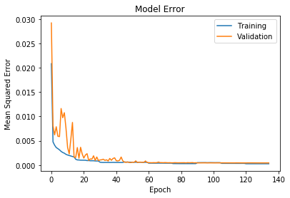
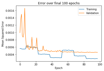
To train the model, the loss was calculated using the mean squared error of the labeled key points and the predicted key points. It was found that the Adam optimizer provided the best results. It was also found that the lowest loss was achieved by progressing the batch size and learning rate. Starting with a learning rate of 0.001, the model was trained for 15 epochs on 32, 64, and 128 batch sizes. This was repeated for learning rates of 0.0001 and 0.00001. The reasoning being that with a lower batch size the gradient descent step is more stochastic(more random) as it is averaged over fewer examples. As the optimization reaches a minimum value the parameter steps should represent a more general solution, provided by taking the average gradient over a larger batch size.
The following figures show the training curves with the latter showing a closer view of the final epochs. As you can see in the final epochs, the steps in the training loss are produced by the increasing batch size for each learning rate.
Pseudo Labeling
After the first round of training, the model is relatively accurate. To make use of all the data in the original dataset, the trained model was used to predict key points for the missing values and use those as labels. Essentially, the dataset had a large amount of incomplete examples that were thrown away, yet they still had useful information from the key points. In order to learn from that information, the model filled in the incomplete points with a best guess.
Taking the pseudo-labeled full dataset and augmenting it as before, a new training dataset was created with 29520 examples. The model then continued training on this data set and was followed by another cycle of training on the original fully-labeled dataset. Ultimately, the model error was trained below 0.0005. I was pretty happy with this as the project notebook stated, “A very good model will achieve about 0.0015 loss”. Furthermore, when plotted on test images, the key point predictions appeared to be placed where you would expect.
Summary
With the key point detection model trained, the face detector and the model were combined to apply key points to faces within an image. The following figure gives an example product of the this process.
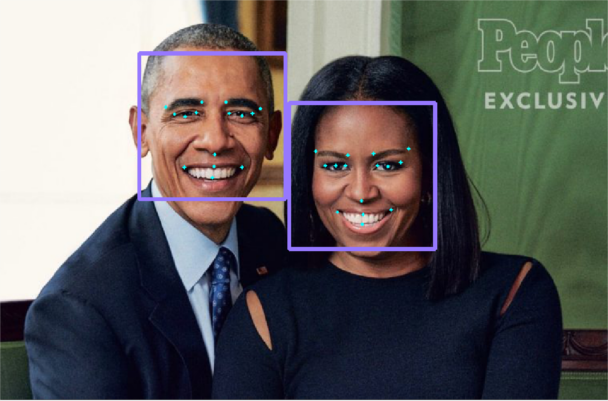
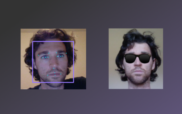
Additionally, the model was extended to work with a web cam and to use the key point features to apply a mask filter(sunglasses in this case).
I was excited with the outcome of this project. Using a simple convolutional architecture with some updated techniques, data augmentation and pseudo-labeling, this model was able to produce useful results on a relatively small dataset.