Neural Translation Model

Overview

In this post, I walk through how to build and train an neural translation model to translate French to English. This post will focus on the conceptual explanation, while a detailed walk through of the project code can be found in the associated Jupyter notebook. This notebook can be viewed here or cloned from the project Github repository, here. This post will be divided into two parts:

1. A Conceptual Understanding of the Model
2. A Brief Summary of How the Model Performed

This project closely follows the PyTorch Sequence to Sequence tutorial, while attempting to go more in depth with both the model implementation and the explanation. Thanks to Sean Robertson and PyTorch for providing such great tutorials.

Understanding the Model

We are trying to build a translation model. One model that has been successful in this task is an Encoder-Decoder network. At a high level, this model takes in a sequence and encodes the information of that sequence into an intermediate representation. This intermediate representation is decoded by the decoder into whatever target language the model has been trained for. In the case of this project, the input sequences are French sentences and the model has been trained to output the English translation of those sentences.

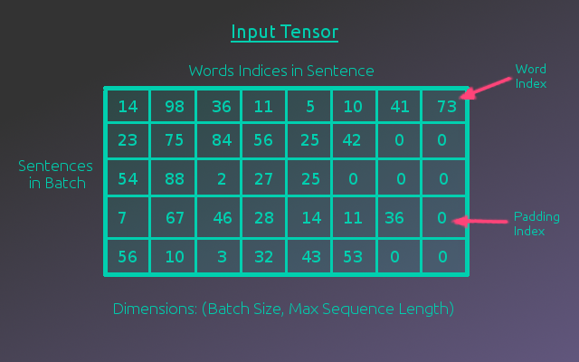
Before we dive into the details of how the encoder and decoder work, we need to have an understanding of how our data will be represented to the model. Without knowing anything about how the model works, we can make the reasonable assumption that if we give the model a sentence in French, it should be able to provide us with the equivalent English sentence. So inputing one sequence of words should output another sequence of words. However, the model is just a collection of parameters that perform various computations on the input. The model does not know what words are. Similar to how letters have a ASCII mapping to numbers, our words need to be represented numerically. To do this, each unique word in the dataset needs a unique index. Rather than a sequence of words, the model will be given a sequence of indices.

This works great for one sentence, but how can we pass the model multiple sentences to speed up the training process? Sentences are not all the same length. Additionally, how will these sequences of numbers be organized for the model? The answer is that the input sequences will be represented as a 2D tensor(matrix) with dimensions (batch size x max sequence length). This allows us to input a batch of sentences and sentences that have a length less than the longest sentence in the dataset can be padded using a pre-determined “padding index”. This is illustrated in the following figure.

Encoder

Word Embeddings

The input tensor allows us to input several sentences to the model as a sequence of indices. This is a step in the right direction, but these indices don’t hold any information. They are just place holders that represent the words. The word represented by the index 54, is not necessarily related to the word represented by the index 55. It wouldn’t make sense to use these index numbers in a calculation. These indices need to be represented in some other format that allows the model to compute something meaningful.

One way to do this is to “one hot encode” the words, meaning each word is represented by a vector of zeros except for a one at the index associated with the word. Each index in this vector would be associated with a unique word in the vocabulary. This would work, but it still lacks any sort of information about how words are related. A better way to represent words is to use word embeddings.

Word embeddings represent each word as an N-dimensional vector. In this way, similar words would have similar word embeddings and would be located near each other in the N-dimensional space. To determine good values for the word embeddings, a model with random word embeddings is trained on some language task. Luckily, this has already been done by other researchers and those word embeddings have been made available. In this project, the 300-dimensional word embeddings from FastText are used.

The indices can now be replaced by the word embeddings associated with each word. This step is included into the Encoder’s calculation giving a third dimension to the input tensor representing the word embeddings. An illustration of this embedded tensor is shown in the following figure.

With the input sentence represented as a sequence of word embeddings and organized into a tensor, it is ready to be feed into the recurrent layer of the Encoder.

Encoder Architecture

As mentioned above, the embedding step is rolled into the Encoder calculation. This is done through an embedding layer. The following figure shows the full Encoder architecture.

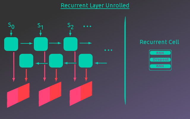
As shown above, once the input tensor has passed through the embedding layer, the embedded input tensor is passed to a Bi-Directional RNN layer. A simple Encoder-Decoder network just uses a forward directional RNN for the encoder. However, this requires that items at the beginning of the sequence be encoded without any information about what is contained later in the sequence. A Bi-Directional RNN avoids this by stepping forward through the sequence as well as backward. As the RNN steps backward through the sequence it has already seen the full sequence.

Taking the embedded input tensor, the RNN steps through each sequence item(word) in the sequence(sentence). At each iteration, an encoding vector with a length equal to the encoder hidden size is output. This is done in parallel for each example in the batch, for that sequence item. Although all the RNN steps are output as one final tensor, it is useful to think of the output at each step as a matrix(batch size X encoder vector size).

At each step through the sequence, the RNN’s hidden state is passed to the next iteration of the RNN that takes in the next sequence item. This iteration also outputs an encoding vector for each example in the batch. This “matrix” is output at each step in the sequence and as the RNN steps backward through the sequence the output matrix is concatenated to the matrix at the same sequence step from the forward pass along the encoded vector dimension. This process is illustrated below. For this project, the RNN cell used 2 layers with one dropout layer between them. Additionally, two different types of RNN’s were compared, LSTM(Long Short Term Memory) and GRU(Gated Recurrent Unit) architectures.

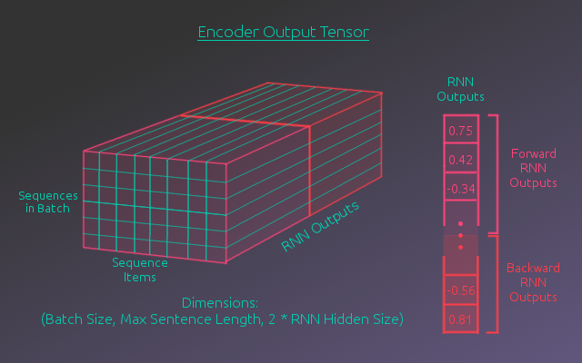
The final output of the RNN layer is a tensor where the “matrix” outputs of each recurrent step are stacked in the sequence dimension. The following figure shows this tensor in detail.

Decoder

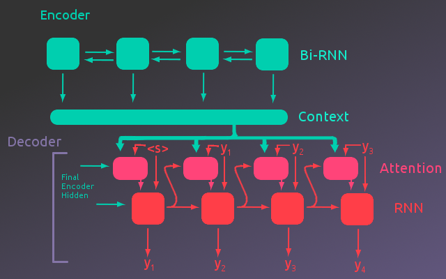
For a simple Encoder-Decoder network the final hidden state of the Encoder is passed to another RNN(The Decoder). Each output from this RNN is a word in the output sequence, which is fed as input to the next step of the RNN. However, this architecture requires that the entire input sequence be encoded into the final hidden state of the Encoder. By using an attentional model, the Decoder takes the final hidden state as well as the Encoder output at each step in the input sequence. The Decoder can then weight the values of the Encoder output that are important for the calculation at each iteration in the Decoder output sequence.

Ultimately, the recurrent layer of the Decoder will take as input, the Encoder Output weighted by the attention module, as well as the predicted word index from the previous step of the recurrent cell. The following figure gives an illustration of this process, where the “Context” represents the Encoder output tensor.(Note that the embedding layers in both models were not included in the illustration to simplify the figure.)

So now let us take a closer look at how the attention module weights the Encoder output.

Attention

Referring back to the Encoder Output Tensor, each item in the sequence dimension holds a vector from the RNN output. This vector is associated with the word at that sequence step, in the input sentence. For each example in a batch, the attention module takes a weighted sum of these vectors across the sequence dimension. This produces one vector, for each example, that represents the relevant information needed for the calculation of the current output sequence step.

To make this explanation a bit more concrete, let’s consider an example. If the first word of the input sentence was the most important piece of information for a given output word, then the weight associated with the first word would be one and all other weights would be zero. This would have the effect that the weighted vector would be equal to the vector associated with the first word from the input sentence.

The model needs to learn how to determine these weights, so a fully connected layer is used to calculate them. There needs to be one weight per word in the sequence, so the number of nodes will equal the maximum sequence length. The weights should also sum to one, so the fully connected layer will use a softmax activation function. To determine these weights, the attention module will take as input, the concatenation of the previous hidden state of the Decoder and the word embeddings of the predicted words from the previous Decoder output step. The following figure illustrates this process.

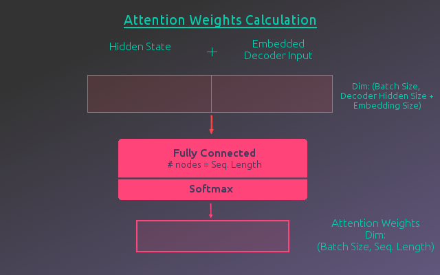
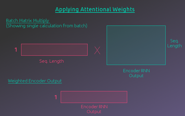
Once the weights are calculated, a matrix multiplication of the weights and the Encoder output, by batch example, will give a weighted sum of the encoded vectors across the sequence. The matrix representing the Encoder output, by batch example, can be thought of as taking a horizontal slice of the Encoder Output Tensor. By writing out this multiplication by hand, you can see that each sequence weight is multiplied by the associated encoded vector and these are summed over the whole sequence to produce a single vector. The following figure illustrates this calculation for a single example. The actual calculation stacks each example in the batch to form a matrix with dimensions (batch size x 2*Encoder Hidden Size). This produces the Weighted Encoder Output.

Recurrent Calculation

Now that the Encoder Output has been weighted by the attention module, it is ready to be passed to the RNN layer of the Decoder. The RNN will also take in the word embeddings of the words predicted by the previous step of the Decoder. Rather than inputing the concatenation of these two matrices straight into the RNN, it will first pass through a fully connected layer with a ReLU activation. The output from this layer will then be the input to the RNN.

The output from the RNN will go through a fully connected layer with a log softmax activation function where the number of nodes is equal to the number of words in the output language vocab. This represents the predictions for the next word in the output sequence. This word along with the hidden state of the RNN are passed to the next step of the attention module and RNN, where the next sequence item is calculated. The following figure illustrates this process. This is repeated until the entire output sequence has been output.

Training the Model

Initially, the model is not very good at predicting the output sequence. It needs to be trained. To do this a loss is calculated and the error is back propagated through the model to update the model parameters. For this model, the loss is calculated by taking the Negative Log Likelihood Loss between the output predictions and the target translation word, summing over the sequence and averaging over the batch. This process is repeated for the entire dataset and for as many epochs of the dataset as needed to obtain the desired results.

However, training a language model is slightly more complicated. Since the Decoder depends on predictions of the previous sequence items to predict later items, an error early in the sequence would throw that whole translation off. This makes it very hard for the model to learn. The solution to this problem is a technique called teacher forcing. The idea is that for some batches(usually half the time, selected at random), instead of passing the previous prediction of the decoder to the next sequence step, the previous target is used. When teaching forcing is used, the calculation of the decoder at each step uses the correct previous word. This technique makes training the model much easier.

Model Performance

The details of building and training this model can be found in the associated Jupyter notebook, which is linked at the beginning of the post. This section will provide a brief summary of how the model performed.

Datasets

Two datasets were used to test the model. The initial dataset used was relatively simple. It had a smaller vocab size and the sentence structure seemed to lack diversity. It did however, have the advantage of training relatively fast while testing out the model. After training on this dataset, a second, more diverse dataset was used. Although this dataset used shorter sentences, it had a much larger vocab size, as well as a much broader sentence structure.

Simple Dataset
Number of examples: 137861

Number of unique French words: 356
Number of unique English words: 228

Longest French sentence: 23 words
Longest English sentence: 17 words

Examples:

French Sentence: paris est jamais agréable en décembre , et il est relaxant au mois d' août .  
English Sentence: paris is never nice during december , and it is relaxing in august .

French Sentence: elle déteste les pommes , les citrons verts et les citrons .  
English Sentence: she dislikes apples , limes , and lemons .

French Sentence: la france est généralement calme en février , mais il est généralement chaud en avril .  
English Sentence: france is usually quiet during february , but it is usually hot in april .

French Sentence: la souris était mon animal préféré moins .  
English Sentence: the mouse was my least favorite animal .

French Sentence: paris est parfois clémentes en septembre , et il gèle habituellement en août .  
English Sentence: paris is sometimes mild during september , and it is usually freezing in august .

More Diverse Dataset
Number of examples: 139692

Number of unique French words: 25809
Number of unique English words: 12603

Longest French sentence: 10 words
Longest English sentence: 10 words

Examples:

French Sentence: je vais laver les plats  
English Sentence: ill wash dishes

French Sentence: les nouvelles les rendirent heureux  
English Sentence: the news made them happy

French Sentence: globalement la conférence internationale fut un succès  
English Sentence: all in all the international conference was a success

French Sentence: comment marche cet appareil photo  
English Sentence: how do you use this camera

French Sentence: cest ton jour de chance  
English Sentence: this is your lucky day

Loss Plots

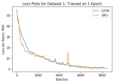
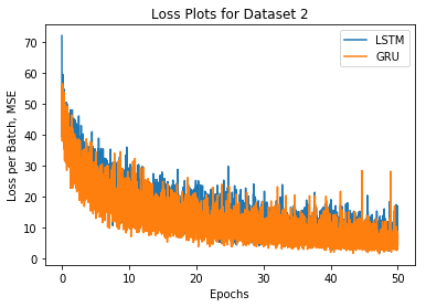
Two versions of the model were built, one using an LSTM cell for the RNN and one using a GRU cell for the RNN. These two versions of the model were trained on the two datasets. Their loss plots are shown below.

Example Translations and Visualizing Attention

Example Translations: Simple Dataset

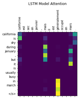
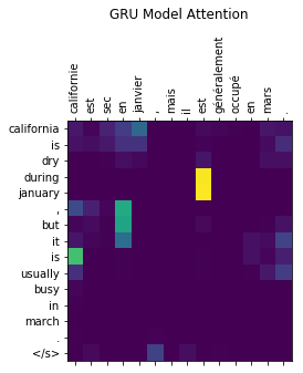
After training the models one epoch on the dataset, both versions were very accurate at producing the correct translation. However, the models did not seem to be using the attention to translate the sequences. Below are 3 example translations and visualizations of the attentional weights at each item in the output sequence. Looking at the examples below, the attention weights are not necessarily random, but the attention is not on the words one would expect.

Example 1

Input Sentence:
 californie est sec en janvier , mais il est généralement occupé en mars . </s>

Target Sentence:
 california is dry during january , but it is usually busy in march .</s>

LSTM model output:
 california is dry during january , but it is usually busy in march . </s>

GRU model output:
 california is dry during january , but it is usually busy in march . </s>

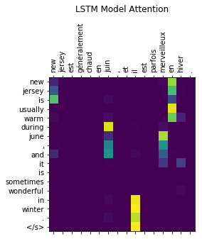
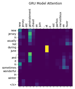
Example 2

Input Sentence:
 new jersey est généralement chaud en juin , et il est parfois merveilleux en hiver . </s>

Target Sentence:
 new jersey is usually hot during june , and it is sometimes wonderful in winter .</s>

LSTM model output:
 new jersey is usually warm during june , and it is sometimes wonderful in winter . </s>

GRU model output:
 new jersey is usually hot during june , and it is sometimes wonderful in winter . </s>

Example 3

Input Sentence:
<unk> les fraises , les mangues et le pamplemousse . </s>

Target Sentence:
i like strawberries , mangoes , and grapefruit .</s>

LSTM model output:
i like strawberries , mangoes , and grapefruit . </s>

GRU model output:
i like strawberries , mangoes , and grapefruit . </s>

Example Translations: More Diverse Dataset

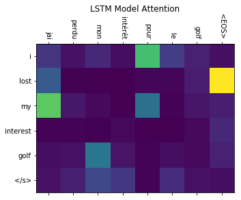
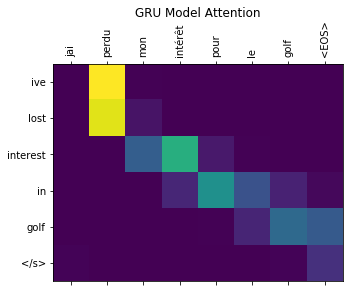
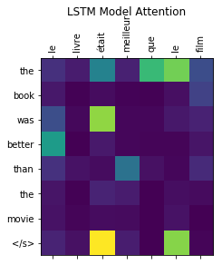
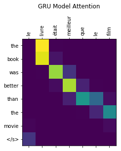
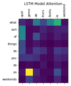
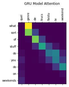
The models were also able to correctly translate the sentences from the more diverse data. However, it took much longer to train, requiring 50 epochs of the data to get reasonable looking results. Several examples can be seen below. The attention weights for the GRU model begin to demonstrate that the model is using the attention mechanism. However, the LSTM model still does not seem to be learning or utilizing attention. This may be due to the LSTM’s access to the cell state which preserves long term dependencies. The attention calculation might not provide enough useful information for the model to prioritize learning better parameters for the attention calculation.

Example 1

Input Sentence:
jai perdu mon intérêt pour le golf </s>

Target Sentence:
ive lost interest in golf</s>

LSTM model output:
i lost my interest golf </s>

GRU model output:
ive lost interest in golf </s>

Example 2

Input Sentence:
le livre était meilleur que le film </s>

Target Sentence:
the book was better than the movie</s>

LSTM model output:
the book was better than the movie </s>

GRU model output:
the book was better than the movie </s>

Example 3

Input Sentence:
 quel genre de trucs <unk> le weekend </s>

Target Sentence:
 what sort of things do you do on weekends</s>

LSTM model output:
 what sort of things do you do on weekends </s>

GRU model output:
 what sort of stuff do you do on weekends </s>

Summary

This model architecture was able to successfully translate the two datasets tested. The GRU model demonstrated that the attention calculation allowed the model to focus on different portions of the encoded sequence. However, it is unclear why the LSTM model appeared to either not make use of the attention information, or use the information in a different way than the GRU model. Given more time, it would have been interesting to investigate why this effect was being observed. Would the effect still be present if a dataset with longer sequences were used? It would also be interesting to compare the model to a simple encoder-decoder network without attention and see what situations the attention model would outperform the simple model, if at all.

The architecture chosen also differed slightly from the model in the Pytorch tutorial that this project followed. The model used for this project allowed for batching of the examples, while the model in the original tutorial was built to process one sequence at a time. Because of this, the original model did not have to deal with padding the output. One would assume that batching would improve training time, by parallelizing the training cycle. However, the claimed training time for the original model was about 40 minutes on a CPU, while it took the model used in this project close to 12 hours, training on GPU, to get good translations.

There are several improvements that might address this discrepancy. First, PyTorch has a built in function to deal with padded sequences so that the recurrent cell doesn’t see the padded items. It is possible that this would improve the models ability to learn. Secondly, the second dataset was not tokenized. Punctuation was just removed, which may have caused some of the words to be unrecognizable when converting the words to indices. This would mean they were replaced with the unknown token, making it harder for the model to identify the content of the sentence. Even though there is room for improvement, overall the project was a success as the model was able to successfully translate French to English.